error: usleep is not declared in this scope

Find every file which have this error and add the codes below to it:

#include <unistd.h>
#include <stdio.h>
#include <stdlib.h>



in case of orbslam2:

Files that need to be added are:

Examples/Monocular/mono_euroc.cc

Examples/Monocular/mono_kitti.cc

Examples/Monocular/mono_tum.cc

Examples/RGB-D/rgbd_tum.cc

Examples/Stereo/stereo_euroc.cc

Examples/Stereo/stereo_kitti.cc

src/LocalMapping.cc

src/LoopClosing.cc

src/System.cc

src/Tracking.cc

src/Viewer.cc

SIFT가 뭐냐

[1] Scale Invariant Feature Transform - David Lowe

1. What is SIFT?
1. Image에서 중요한 feature points를 찾는 기술
2. Features?: 포인트 주변을 잘 설명해주는 정보. rotation, scale과 관련 있음
2. Motivation for SIFT
1. Image matching
1. 이미지들 사이의 affine transformation과 homography를 추정하는 것
2. Fundamental matric in stereo 추정 (카메라 여러대?)
2. Motion, tracking, motion segmentation의 구조 파악
3. 이미지들의 중요하고 stable한 points 찾기 & 이것들 사이의 관계 결정하기
4. Feature는 물체 위치, 자세, 스케일, 조도, 노이즈 등에 무관해야 함
5. Individual pixel colour values are not an adequate feature to determine correspondences (?)

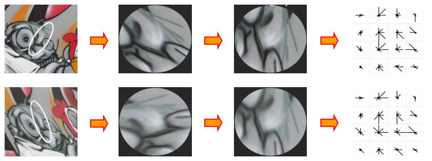
SIFT는 변화(회전이나 스케일)에 관계없이 feature를 잘 찾아냄. 위의 그림에서 같은 것으로 잘 인식하는 것을 볼 수 있음. (서로 다른 두 이미지에서 SIFT특징을 각각 추출한 다음에 가장 비슷한 특징끼리 매칭해주면 두 이미지에서 대을되는 부분을 찾을 수 있음.)

3. Steps of SIFT algorithm
1. Step 1) Scale Space 만들기
1. Scale Space란?
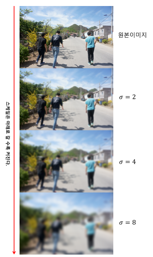
1. 영상처리를 할 때 단 하나의 스케일을 가진 이미지가 아니라 여러 스케일로 본 이미지들을 가지고 작업하는 것 -> 이 이미지 뭉치가 바로 Scale Space
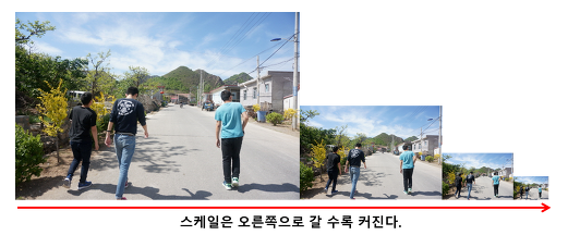
2. 스케일이 커질수록 디테일한 것이 잘 안보임 -> 이미지 사이즈는 유지하면서 blur처리를 하면 스케일이 커진 것과 같은 효과를 볼 수 있음
1. Blur처리를 어떻게 하는지? -> Gaussian Filter를 이용한다.

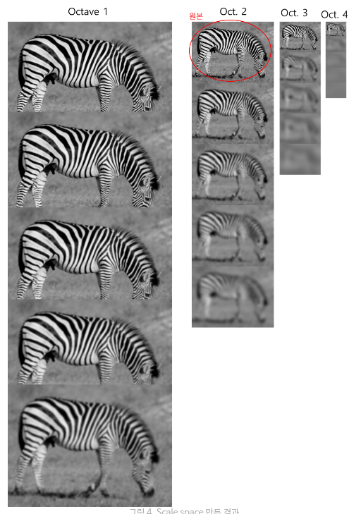
2. 스케일 파라미터 σ가 커질수록 스케일이 커진다.
2. 원본 이미지를 2배, 1/2배, 1/4배로 만들어서 스케일 파라미터를 다르게 총 4세트를 만든다.
3. 이게 바로 Scale Space
2. Step 2) DoG 연산 (Difference of Gaussian)
1. Laplacian of Gaussian(LoG)를 이용해서 이미지 내의 key points를 찾는다.
1. Blur -> 2차미분
2. but, 이 녀석은 계산이 너무 많음
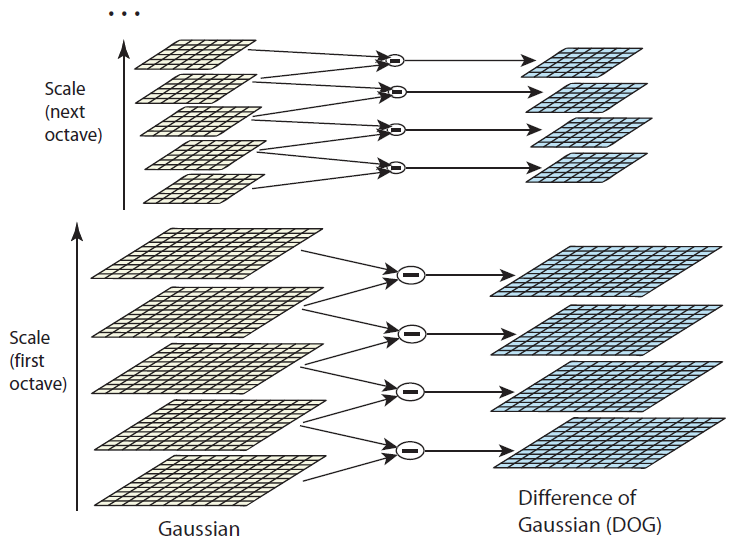
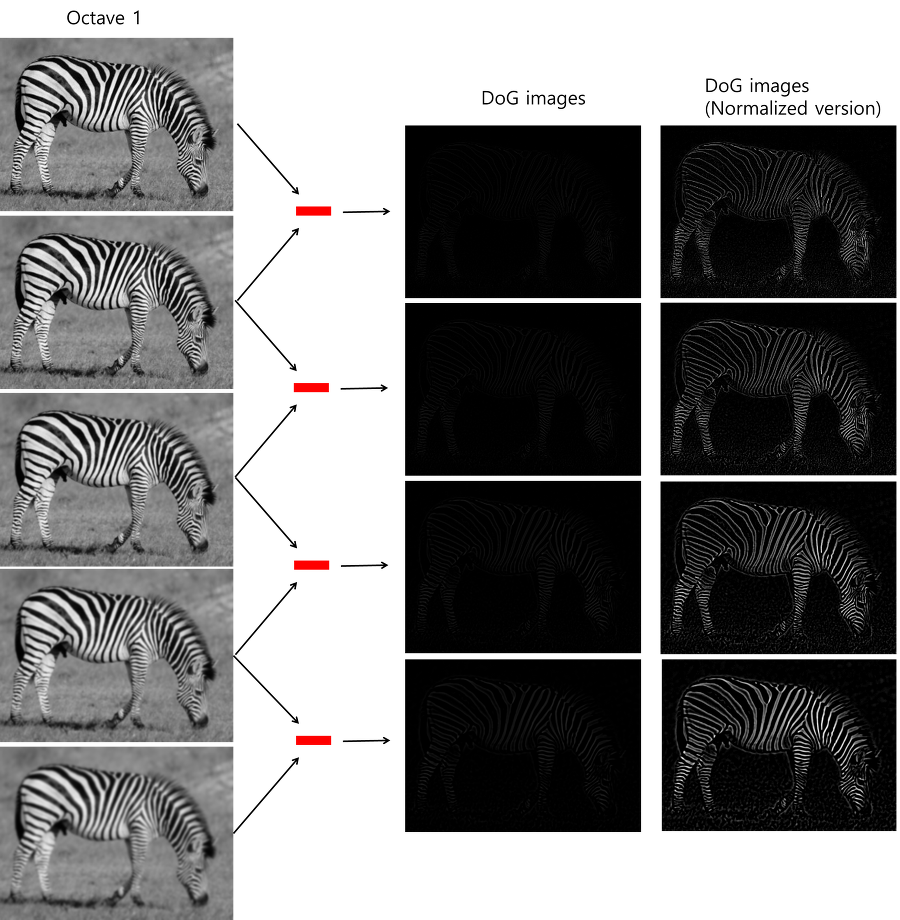
2. Difference of Gaussian(DoG)
1. 라플라시안을 구하는 것을 컨볼루션을 해야하지만, DoG는 화소값의 차이만 구하면 되므로 계산이 수십배에서 수백배로 빨라짐.
2. 같은 옥타브 내에서 인접한 두개의 블러 이미지들끼리 빼줌
3. 
4. 
3. Step 3) Key point들 찾기
1. 한 픽셀에서 극대값, 극소값을 결정할 때는 동일한 octave내의 3장의 DoG이미지가 필요함. 지금 체크할 픽셀 주변의 8개 픽셀과, scale이 한단계씩 다른 위 아래 두 DoG 이미지에서 체크하려고 하는 픽셀과 가까운 9개씩, 총 26개를 검사합니다. 만약 지금 체크하는 픽셀의 값이 26개의 이웃 픽셀값 중에 가장 작거나 가장 클 때 keypoint로 인정.
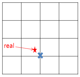
2. 테일러 2차 전개를 이용, 픽셀 사이의 정확한 키 포인트를 찾아낸다.
4. Step 4) 나쁜 Key point들 제거하기
1. 활용가치가 떨어지는 것들을 제거
1. 낮은 콘트라스트를 가지고 있거나(threshold 이하)
2. 엣지 위에 있는 것
2. 코너에 있는 키포인트들이 좋은 것임
5. Step 5) key points에 방향 할당해주기
1. 지금까지 얻은 키포인트는 scale invariance를 만족, 지금부터는 rotation invariance를 위한 것.
2. Key point 주변의 그래디언트 방향과 크기를 활용, 가장 큰 그래디언트의 방향이 키포인트의 방향이 된다.
6. Step 6) 최종 SIFT 특징 산출
1. 지금까지 얻은 키포인트들은 scale, rotation 불변성을 가지고 있음
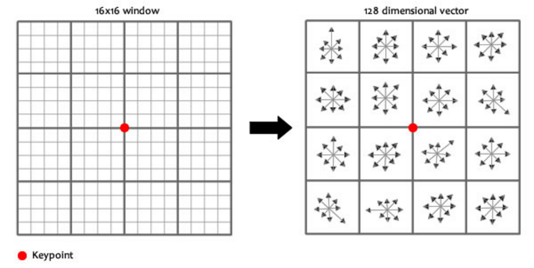
2. 이것들을 식별하기 위한 정보(지문) 부여(그래디언트의 크기와 방향)
1. 
3. 그렇다면 SIFT로 이미지 매칭을 어떻게 하는 것일까요? 먼저 두 이미지에서 각각 keypoint들을 찾고 지문을 달아줬다면, 이 지문값들의 차이가 가장 작은 곳이 서로 매칭되는 위치인 것입니다.
2. 장단점
1. 장점
1. Affine transformation에 강건
2. Illumination changes에 강건
2. 단점
1. 3D 물체보다 평면에서 작동이 잘됨
2. Several parameters in the algorithm: descriptor size, size of the region, various thresholds – theoretical treatment for their specification not clear

FAST알고리즘을 이용한 특징 검출

FASTER and better: A machine learning approach to corner detection

FAST알고리즘을 이용한 특징 검출

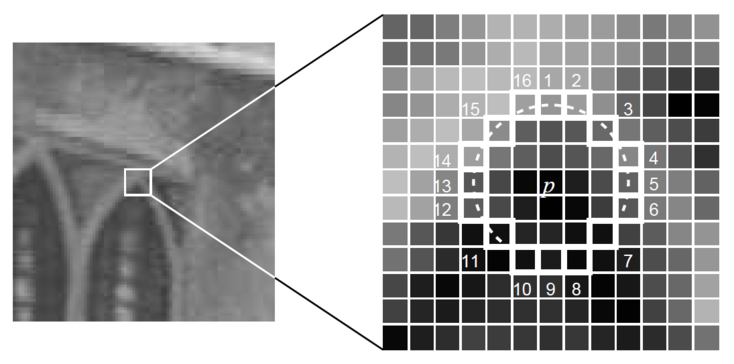
1. 이미지에서 픽셀 p를 선택. 이 때, 선택한 p의 밝기는 Ip.
2. 적당한 threshold t를 정함.
3. p주위의 원 내부에 lp+t보다 밝은 픽셀이 n개 연속으로 존재하거나, Ip-t 보다 어두운 픽셀이 n개 연속으로 존재하면 픽셀 p를 코너로 판단. (논문에서 n은 12)
1. 

이 detector는 아주 좋은 성능을 보여주지만, 몇가지 단점이 있음

1. This high-speed test does not reject as many candidates for n < 12 since the point can be a corner if only two out of the four pixels are both significantly brighter or both significantly darker than p (assuming the pixels are adjacent). Additional tests are also required to find if the complete test needs to be performed for a bright ring or a dark ring.
1. 과연 12라는 n이 적당한가?
2. The efficiency of the detector will depend on the ordering of the questions and the distribution of corner appearances. It is unlikely that this choice of pixels is optimal.
1. p를 어떻게 선택할 것인가?
3. Multiple features are detected adjacent to one another.
1. p주위로 여러 features들이 나타날 수 있지 않는지?

이 약점 세가지는 machine learning으로 극복할 수 있음

1. 코너 검출을 위한 machine learning
1. Training을 위한 image dataset 선택
2. Features를 찾기 위해 모든 이미지에 FAST 알고리즘 실행
3. 검출된 모든 픽셀에 대해 픽셀 주위로 16개 픽셀을 벡터로 저장 (이 벡터를 P라고 하자)
4. 그렇다면 그 픽셀들은 이렇게 나타낼 수 있음:
1. 이 함수에 따라 벡터 P는 Pd(darker), Ps(similar), Pb(brighter)로 나타낼 수 있음
2. 이것으로 새로운 boolean 변수 Kp를 정의 -> p가 코너면 true, 아니면 false
3. Pd, Ps, Pb에 Kp변수를 이용해 코너를 빠르게 검출하는 의사결정 트리 생성
2. Non-maximal Suppression
1. 검출된 feature points에 대해 p와 주변 픽셀 16개의 차 절대값을 모두 더한 값인 V 계산
2. 인접한 2개의 key point의 V를 비교해 작은 것을 버린다.

한계!

FAST는 아주 빠르지만 노이즈가 많으면 잘 안되고, threshold 값에 의존적임…

SLAM

References

1. R. Mur-Artal, J. M. M. Montiel, and J. D. Tardos, “ORB-SLAM: A versatile and accurate monocular SLAM system,” IEEE Transactions on Robotics, vol. 31, no. 5, pp. 1147–1163, Oct. 2015.

In this paper, the authors suggest the new algorithm for simultaneous localization and mapping called ORB-SLAM. It is the feature based monocular SLAM system in a small or large environment and in both indoor and outdoor. The main idea of this paper is using PTAM that means parallel tracking and mapping and loop closing. PTAM is the one of visual SLAM algorithm that uses keyframes and the differences between them.

ORB-SLAM reduced the calculating time of each image a lot but it seems that the tracking accuracy can be higher. Also, it only makes the sparse map but it can be the good root for the further algorithm to make the dense map.

This paper is relevant to my current topic because this is the one of most famous SLAM until now and I want to improve SLAM in self-driving car field.

2. D. Detone, T. Malisiewicz, and A. Rabinovich, “SuperPoint: Self-supervised interest point detection and description,” in 2018 IEEE/CVF Conference on Computer Vision and Pattern Recognition Workshops (CVPRW), Apr. 2018.

In this paper, the authors turned the deep learning into the frontend of the SLAM system. There is a shared encoder to keep the model fast and easy to train which is operated by the interest point decoder for detection and the descriptor decoder for description.

This paper used self-supervised learning so it worked well even in so many diversion of views and lights as compared with classic feature extracting and matching algorithms.

The attempt to combine with deep learning and the feature extraction can be a good frame to my further work to make the end-to-end neural network model for SLAM.

3. E. Parisotto, D. S. Chaplot, J. Zhang, and R. Salakhutdinov, “Global pose estimation with an attention-based recurrent network,” in 2018 IEEE/CVF Conference on Computer Vision and Pattern Recognition Workshops (CVPRW), Feb. 2018.

In this paper, the authors turned the deep learning into the backend of the SLAM system. The main concept of this paper is the neural global optimizer consist of local pose estimation model, pose aggregation module and neural graph optimization. It predicts the relative pose changes and optimizes the predictions.

This paper was the first attempt to use deep learning in SLAM. Although it is not the end-to-end model, it is well worth enough. They have the enormous potential for development because there are several convolutional network models can be applied instead of Flownet that it used in this paper.

The neural global optimizer is one of good related work for my further work to make the end-to-end neural network model for SLAM.

4. G. Klein and D. Murray, “Parallel tracking and mapping for small AR workspaces,” 2007 6th IEEE and ACM International Symposium on Mixed and Augmented Reality, 2007.

Original visual SLAM considers every frame to pick feature points but Parallel Tracking and Mapping(PTAM) picks them in keyframes so it is faster than before. It runs tracking and mapping separately in parallel threads. There are few calculations in tracking so it is applied on every video frames for making it real-time and more accurate but mapping is applied on only keyframes.

However, PTAM is appropriate to apply only in fixed and limited space like the office desk. Also, there is no loop detection which makes the result more accurate and the user should do the initialization for scaling before running the algorithm.

This work became the base work of ORB-SLAM.

5. S. Milz, G. Arbeiter, C. Witt, B. Abdallah, and S. Yogamani, “Visual SLAM for automated driving: Exploring the applications of deep learning,” in 2018 IEEE/CVF Conference on Computer Vision and Pattern Recognition Workshops (CVPRW), 2018.

In this paper, authors did the brief summary of some important SLAM algorithms so far, introduced the fundamental pipeline of SLAM and explained how and why deep learning can help them to improve. Also, there are short descriptions about considering problems in self-driving vehicles field.

Because this paper is written in early 2018 there is no important researches of 2018 and 2019 so far but it is helpful to read quickly about classical visual SLAM approaches such as PTAM, ORB-SLAM and Mono SLAM.

There is slow development on convolutional neural network based SLAM algorithm approaches. This paper helped me to learn SLAM briefly and gave me some insights of adopting deep learning to it.

6. Kang Rong, Jieqi Shi, Xueming Li, Yang Liu and Xiao Liu. "DF-SLAM: A deep-learning enhanced visual SLAM system based on deep local features." arXiv preprint arXiv:1901.07223, 2019.

DF-SLAM is proposed with the deep local feature descriptors adopted by the neural network which can replace ORB, SIFT or other classic feature descriptors. This system runs three threads in parallel, there are tracking, local mapping and loop closing each. The new local feature descriptors are extracted before the tracking thread manages a new frame.

DF-SLAM can be more stable. Also, there is a limitation that it is hard to handle difficult localization and mapping problems under extreme conditions. There are some points to improve include global bundle adjustment.

This paper can help me to establish the end-to-end system for deep learning enhanced and powerful SLAM algorithm.

Install PyCharm in Ubuntu using umake

Install PyCharm in Ubuntu using umake

Ubuntu provides a wonderful command line tool, umake for developers. umake lets you easily install a number of development tools in Ubuntu such as Android Studio, Visual Studio Code, Ubuntu SDK, Eclipse, Arudino Software Distribution etc. PyCharm is also one of the development tools included in the umake.

To install PyCharm using umake, you need to have umake first. Normally, it should already be installed in your system, but if it is not, use the PPA below to get the latest stable version of umake:

sudo add-apt-repository ppa:ubuntu-desktop/ubuntu-make
sudo apt-get update
sudo apt-get install ubuntu-make

Once you have umake, use the command below to install PyCharm Community Edition in Ubuntu:

umake ide pycharm

To install PyCharm Professional Edition (you need a license for this), you can use the command below:

umake ide pycharm-professional